Quantum Fourier Transformation
Can one implement Fourier transform on a quantum computer? Can this help us decompose our music into fundamental frequencies even faster? What if I say the answer to the former is ‘yes’ but latter is ‘no’. Read this blog post to know why and how.
Prerequisites: This blog post assumes the reader is familiar with discrete Fourier transformation(DFT) and basics of quantum computing. To get an introduction into DFT check out my blog post - Discrete Fourier Transforms.
Quantum Fourier Transformation (QFT)
Similar to DFT definition, QFT on an orthonormal basis $|0\rangle \dots |N-1\rangle$ is defined to be a linear operator with the following action on the basis states,
\(QFT |j\rangle = \frac{1}{\sqrt{2^n}}\sum_{k=0}^{2^n-1}e^{2\pi ijk/2^n}|k\rangle\) The action on an arbitrary state may be written as
\[\sum_{j=0}^{N-1} x_j|j\rangle = \sum_{k=0}^{N-1} y_k |k\rangle\]where $y_k$ are DFT of the amplitudes $x_j$. This expression strengthens our understanding of the basis transformation nature of the algorithm. Notice that though the definition of DFT and QFT are similar we can not use QFT to replace DFT in classical computing. As though QFT computes the Fourier transform of $|j\rangle$, once we measure the summation collapses to one value of k.
Pause and ponder: Is the above defined transformation unitary? How will you prove that? Click to expand
Claim: \(U\) is Unitary
\[U^{+} U=\frac{1}{N}\left(\sum_{k=0}^{N-1} e^{-2 \pi i j \cdot k / N}\langle k|\right)\left(\sum_{k^{\prime}=0}^{N^{-1}} e^{+2 \pi i j \cdot k' / N}|k'\rangle\right)\] \[=\frac{1}{N} \sum_{k=0}^{N-1} \sum_{k^{\prime}=0}^{N-1} e^{\frac{2 \pi i j}{N}\left(k^{\prime}-k\right) j}\left\langle k \mid k^{\prime}\right\rangle\]\(=\frac{1}{N} \sum_{k=0}^{N-1} \mathbb{I} \cdot 1=\frac{N}{N} \mathbb{I}=\mathbb{I}\)
Though it is not obvious from the definition of QFT, but this transformation is a unitary transformation and thus can be implemented as the dynamics for a quantum computer. The theorem below will show this fact and also give an expression that can be easily interpreted when designing a quantum circuit for the QFT algorithm.
We consider $N= 2^n, n \in \mathbb{Z}$. As earlier, the basis $|0\rangle \dots |N-1\rangle$ is $|0\rangle \dots |2^n -1\rangle$ thus can be represented using $n$ bit-string. Thus, $|j\rangle = |j_1 \dots j_n\rangle$ where $j = j_1 2^{n-1} + j_2 2^{n-2} + \dots + j_n 2^0$. Also $0.j_lj_{l+1} \dots j_m$ is binary fraction $\frac{j_l}{2} + \frac{j_l}{2^2} + \dots + \frac{j_m}{2^{m-l+1}}$.
One can show that
\[|j_1, \dotsc, j_n\rangle \xrightarrow{QFT} \frac{1}{2^{n/2}} \left[ \left( |0\rangle + e^{2\pi i 0.j_n} |1\rangle \right) \left( |0\rangle + e^{2\pi i 0.j_{n-1} j_n} |1\rangle \right) \cdots \left( |0\rangle + e^{2\pi i 0.j_1 j_2 \dotsm j_n} |1\rangle \right) \right]\]Pause and ponder: How to prove the above? Click to expand
\(=\frac{1}{2^{n/2}}\left[|0\rangle + e^{2\pi i0.j_n}|1\rangle) (|0\rangle + e^{2\pi i0.j_{n-1}j_n}|1\rangle) \dotsm (|0\rangle + e^{2\pi i0.j_1j_2 \dotsm j_n}|1\rangle\right]\)
Pause and ponder: Is there any relation between QFT and Hadamard transformation? Click to expand
Consider
\[U|00\ldots 0\rangle\]where \(U\) is QFT
\[=\frac{1}{\sqrt{N}} \sum_{k=0}^{N-1} e^{2 \pi i j k / N}|k\rangle\] \[=\frac{1}{\sqrt{N}} \sum_{k=0}^{N-1} 1 \cdot | k\rangle\]The coefficients have become 1 as \(j \cdot k=j_1 \cdot k_1+j_2 \cdot k_2 \cdots j_N \cdot k_N = 0\)
So, \(U|00\ldots 0\rangle =\frac{1}{\sqrt{N}} \sum_{k=0}^{N-1}|k\rangle\) which is the equal superposition of all basis, which is nothing but Hadamard on \(|00\ldots 0\rangle\).
Quantum circuit for implementing QFT
Let the gate $R_k$ denote the unitary transformation, \(R_k \equiv \begin{pmatrix} 1 & 0 \\ 0 & e^{\frac{2\pi i}{2^k}} \end{pmatrix}\)
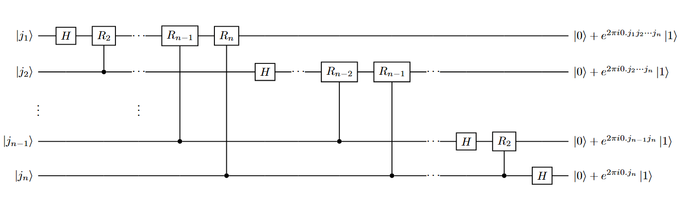
Consider the state $|j_1 \dotsm j_n\rangle$ is input. Applying the Hadamard gate to the first bit produces the state
\[\frac{1}{\sqrt{2}} \left(|0\rangle + e^{2\pi i0.j_1} |1\rangle \right) |j_2 \dotsm j_n\rangle,\]since $e^{2\pi i 0.j_1} = -1$ when $j_1 = 1$, and is $+1$ otherwise. Applying the controlled $R_2$ gate produces the state,
\[\frac{1}{\sqrt{2}} \left( |0\rangle + e^{2\pi i 0.j_1 j_2} |1\rangle \right) |j_2 \dotsm j_n\rangle.\]We continue applying the controlled $R_3$, $R_4$ through $R_n$ gates, each of which adds an extra bit to the phase of the coefficient of the first $|1\rangle$. At the end of this procedure, we have the state,
\[\frac{1}{\sqrt{2}} \left( |0\rangle + e^{2\pi i 0.j_1 j_2 \dotsm j_n} |1\rangle \right) |j_2 \dotsm j_n\rangle.\]Next, we perform a similar procedure on the second qubit. The Hadamard gate puts us in the state,
\[\frac{1}{\sqrt{2^2}} \left( |0\rangle + e^{2\pi i 0.j_1 j_2 \dotsm j_n} |1\rangle \right) \left( |0\rangle + e^{2\pi i 0.j_2} |1\rangle \right) |j_3 \dotsm j_n\rangle,\]and the controlled-$R_2$ through $R_{n-1}$ gates yield the state,
\[\frac{1}{\sqrt{2^2}} \left( |0\rangle + e^{2\pi i 0.j_1 j_2 \dotsm j_n} |1\rangle \right) \left( |0\rangle + e^{2\pi i 0.j_2 \dotsm j_n} |1\rangle \right) |j_3 \dotsm j_n\rangle.\]We continue in this fashion for each qubit, giving a final state,
\[\frac{1}{\sqrt{2^n}} \left( |0\rangle + e^{2\pi i 0.j_1 j_2 \dotsm j_n} |1\rangle \right) \left( |0\rangle + e^{2\pi i 0.j_2 \dotsm j_n} |1\rangle \right) \dotsm \left( |0\rangle + e^{2\pi i 0.j_n} |1\rangle \right).\]Swap operations (which are not shown in the figure) are then used to reverse the order of the qubits, which are simple transmutations of the elements leading to a reverse peruation. After the swap operations, the state of the qubits is,
\[\frac{1}{\sqrt{2^n}} \left( |0\rangle + e^{2\pi i 0.j_n} |1\rangle \right) \left( |0\rangle + e^{2\pi i 0.j_{n-1} j_n} |1\rangle \right) \dotsm \left( |0\rangle + e^{2\pi i 0.j_1 j_2 \dotsm j_n} |1\rangle \right).\]Comparing with the above modified QFT expression derived from the definition of QFT, we see that this is the desired output from the quantum Fourier transform. This construction also proves that the quantum Fourier transform is unitary since each gate in the circuit is unitary.
How many gates does this circuit use? We start by doing a Hadamard gate and $n - 1$ conditional rotations on the first qubit which is a total of $n$ gates. This is followed by a Hadamard gate and $n-2$ conditional rotations on the second qubit, for a total of $n + (n-1)$ gates. Continuing in this way, we see that $n+(n-1)+\dots+1 = \frac{n(n+1)}{2}$ gates are required, plus the gates involved in the swaps. At most $\frac{n}{2}$ swaps are required, and each swap can be accomplished using three controlled-$X$ gates. Therefore, this circuit provides a $O(n^2)$ algorithm for performing the quantum Fourier transform.
In contrast, the best classical algorithms for computing the discrete Fourier transform on $2^n$ elements are algorithms such as the Fast Fourier Transform (FFT), which compute the discrete Fourier transform using $O(n 2^n)$ gates. That is, it requires exponentially more operations to compute the Fourier transform on a classical computer than it does to implement the quantum Fourier transform on a quantum computer.
FFT from DFT
DFT takes $\Theta(2^{2n})$ operations on an input with $2n$ components. This is quite easy to see if we look at the $2^n \times 2^n = 2^{2n}$ matrix of DFT:
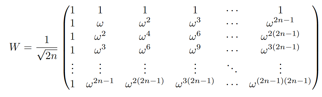
If we multiply $W$ with a vector and count the operations, we get the result.
The modified QFT expression allows you to take advantage of the fact that the Fourier transformed $|j_1,j_2,\dotsc,j_n\rangle$ is made out of $n$ tensored $2 \times 1$ vectors. So, we process each $2 \times 1$ vector independently by performing the following $n$ mappings:
\[\frac{1}{\sqrt{2}} \begin{pmatrix} |0\rangle + |1\rangle \\ \vdots \\ |0\rangle + |1\rangle \end{pmatrix} \rightarrow \frac{1}{\sqrt{2}} \begin{pmatrix} |0\rangle + e^{2\pi i 0.j_n}|1\rangle \\ \vdots \\ |0\rangle + e^{2\pi i 0.j_1\dotsc j_n}|1\rangle \end{pmatrix}\]Each mapping takes a constant number of operations in $n$ as it is simply multiplying a $2 \times 1$ vector by a $2 \times 2$ phase matrix.
\[R_k = \begin{pmatrix} 1 & 0 \\ 0 & e^{\frac{2\pi i}{2^k}} \end{pmatrix}\]Hence, we perform $n$ matrix-vector multiplication to process a single $|j_1\dotsc j_n\rangle$.
We know that an arbitrary vector $|\psi\rangle$ on $n$ qubits can be written as a linear combination of $2^n$ binary kets $|j_1,j_2,\dotsc,j_n\rangle$. For example, for $n=2$, an arbitrary state can be written as a linear combination of $2^2$ binary kets as follows:
\[|\psi\rangle = a|00\rangle + b|01\rangle + c|10\rangle + d|11\rangle\]Therefore, to transform $|\psi\rangle$ on $n$ qubits, we need to process $2^n$ binary vectors $|j_1,\dotsc,j_n\rangle$ by performing $n$ mappings described above. Since each such binary vector requires $n$ matrix-vector multiplications, and there are $2^n$ of them, it takes $\Theta(n2^n)$ operations.
References
[2] Rajat Mittal. Quantum fourier transform. Lecture notes.