As ingenious as RSA is, Shor’s Algorithm is equally remarkable—with the potential to break it and disrupt modern secure systems. This blog post offers a detailed and engaging introduction to Shor’s Algorithm, exploring its implications for cryptography.

Prerequisites: This blog post assumes the reader is familiar with basic group theory, RSA cryptography and quantum Fourier transform. For the ones who are not familiar with RSA can check out my previous blog post - RSA Cryptography. To understand quantum Fourier transform you can refer to my blog post - Quantum Fourier Transform.

In the previous blog post we saw the power of Public Key Cryptography and looked into the detailed description of RSA. The success of RSA relies on the computational hardness of the discrete logarithm problem. More precisely we saw that the real difficulty was in factoring $N$ (a really large number) to its prime factors $P$ and $Q$. In this post we will see how this is no more a barrier when we have access to a quantum computer. The Shor’s algorithm gives us the power to do this.

One thing to note is that, Shor’s algorithm does not allow us to factor a number directly. Instead, it allows us to find the order of an element $a$ modulo $n$ in polynomial time. We will see that finding a factor of $n$, given the order of some element in $\mathbb{Z}/n\mathbb{Z}$ can be done efficiently even on a classical computer, but no efficient algorithm is known for finding the order of the element.

Like we did in the previous blog post here as well we will take a detour into number theory to understand the basis of Shor’s algorithm.

More on Number Theory

With a number theoretic lens one will be able to see that the problem of finding a non-trivial factor to $n$ can be reduced (efficiently) to finding the order of a non-trivial element in $\mathbb{Z}/n\mathbb{Z}$.

Lemma: Given a composite number $n$, and $x$ non-trivial square root of $1$ modulo $n$, i.e. $x^2 \equiv 1$ $\mod{N}$ but $x$ is neither $1$ nor $-1\mod{n}$, then either $\gcd(x-1, \ n)$ or $\gcd(x+1, \ n)$ is a non-trivial factor of $n$.

Proof: Since $x^2\equiv1\mod{n}$, we have $x^2 - 1 \equiv 0\mod{n}$. Factoring, we get $(x - 1)(x + 1) \equiv 0\mod{n}$. This implies that $n$ is a factor of ($x$ + 1)($x - 1$). Since $(x \pm 1) \not\equiv 0\mod{n}$, $n$ has a non-trivial factor with $x$ + 1 or $x-1$. To find this common factor efficiently, we apply Euclid’s algorithm to get $\gcd(x-1, \ n)$ or $\gcd(x+1, \ n)$.

Example: Let $n = 55 =5\times 11$. We find that $34$ is a square root of $1\mod n$ since $342 = 1156 = 1 + 21 \times 55$. Computing, we get $\gcd(33,\ 55) = 11$ and $\gcd(35, 55) = 5$.

This is enough number theory background to straight away jump into Shor’s algorithm.

Overview of Shor’s Algorithm

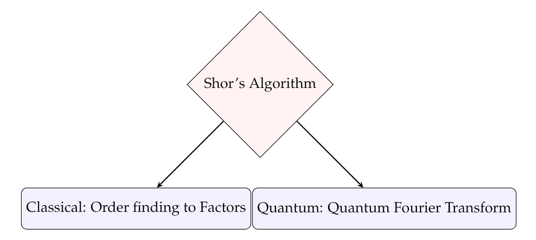
Shor’s algorithm consists of a classical and a quantum part.

Classical Part of Shor’s Algorithm

From the above number theory background we note that, given a composite number $n$ and the order $r$ of some $x \in \mathbb{Z}/n\mathbb{Z}$, we can compute $\gcd(x^{r/2} \pm 1, n)$ efficiently using Euclid’s algorithm. This gives a non-trivial factor of $n$ unless $r$ is odd or $x^{r/2} \equiv -1 \mod{n}$.

Shor’s Algorithm Pseudo-code:

Input: $N = PQ$ where $P$ and $Q$ are primes

Output: $P, Q$

• Pick a number $a$ that is coprime with $N$ i.e. their gcd is 1.
• Find the order $R$ of the function $a^R \mod N$.
• If $R$ is even:
  • Define $x \equiv a^{R/2} \mod N$
  • If $x + 1 \not \equiv 0 \mod N$: Then the factors $P$ and $Q$ which we are looking for, at least one of them is contained in ${\gcd(x+1, N), \ \gcd(x-1, N)}$
  • If either of the above two conditions fails, then pick another $a$ and repeat this all over again.

Remark: Note that given $a^R = 1 \mod N$ and $r$ is even we can factor $a^R-1$ as $(a^{\frac{R}{2}}-1)(a^{\frac{R}{2}}+1)=0 \mod N$. If $x \equiv a^{R/2} \mod N$, then possibly either $x-1$ or $x+1$ divides $N$. But note that the former is not possible as we started with the assumption that the orbit of $a$ is of size $R$, so it can not be $R/2$. If $x+1$ divides $N$ we just repeat the process again (as said in point 4.)

If both the above fails, then either $x-1$ or $x+1$ is a multiple of $Q$ and $P$, where $N=QP$. Thus finding ${\gcd(x+1, N), \ \gcd(x-1, N)}$ gives $P$ and $Q$.

Let us see an example, to kept it really simple say $N=15$ (Note that in reality RSA uses really huge primes. Here we take 25 just for illustration purpose.)

Consider factoring 15:

• Let us pick $a= 13$, as 13 is coprime with 15.
• We need to find the order of $13^x$$\mod{15}$.

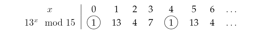
• Since $R$ is the smallest number such that $a^r \equiv 1 \mod{N}$, here $r=4$ since the values are periodic about $x=0,4,8,\dots$.
• $R=4$ is even, define $x = a^{R/2}\mod{N}= 13^{4/2}\mod{15}= 13^2\mod{15}= 4\mod{15}$. Therefore, $x \equiv 4\mod{15}$, hence $x + 1 \equiv 4 + 1\mod{15}\equiv 5\mod{15}\not \equiv 0\mod{15}$. This implies $P$ or $Q$ is in ${\gcd(x + 1, \ N),\ \gcd(x - 1,\ N)}$. Here $\gcd(4+1,\ 15),\ \gcd(4-1,\ 15) = 5,\ 3$. So, $P=5$ and $Q=3$.

Why can not we implement the above algorithm completely classically? The reason is that it becomes progressively harder to find the order (it takes exponential running time). We can see this by looking at the plot between $a^{z} \mod{N}$ and $z$. As the number $N$ grows, the period grows very quickly, and this function appears more and more aperiodic. For $N = 314191$, classical computer runs for about 2 hours in real-time computing. This order-finding part is expedited by using quantum computers.

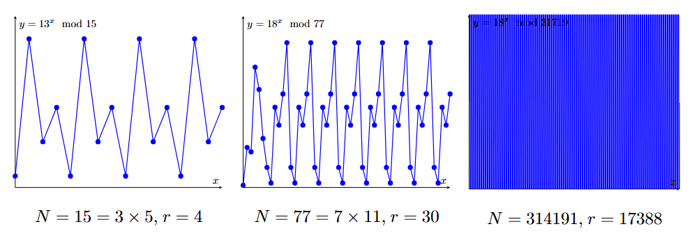
Click here to get the Python code to generate the above plots for your favorite number and check for yourself how fast the run time grows as the numbers become larger. Also you can run the whole Shor’s algorithm in classical computer but it will run very slow for large numbers (click here to explore).

So now the actual task is to find the order $r$ of some $x \in \mathbb{Z}/n\mathbb{Z}$. This is where quantum computing in the form of quantum Fourier transform comes into play.

Quantum Part of Shor’s Algorithm

For the following section, we will assume that $N’$ is a composite odd integer which is not a power of prime (the algorithm fails otherwise). If $N’$ is even, we can just factor out all the powers of 2 until we get an odd integer, then run the algorithm on the resulting integer. We can test whether $N’$ is a prime efficiently using classical primality tests such as the AKS test and the Miller-Rabin test (links to further reading about these is given below in the references. The AKS test was an outcome of a phenomenal papers by outstanding Indian Computer Scientists, especially 2 of the 3 authors of the papers were young under-graduate students). We can also test if $N’$ is a power of prime efficiently by taking the $k$th root of $N’$ until $\sqrt[k]{N’} < 2$.

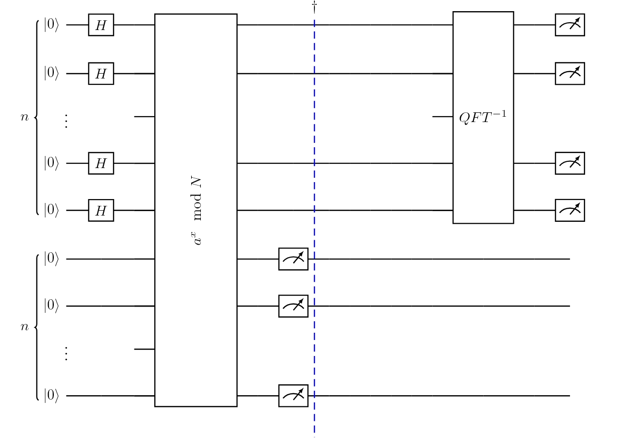
Given $N’$, we choose $N = 2^n$ such that $N’ < N < 2N’$ (i.e., choose the unique power of 2 in that range). We will be working with two registers (two arrays of qubits), such that each of them holds $n$ qubits. At first, both the registers are in state 0.

We put the first register in the uniform superposition of numbers $x\mod{N}$ by using the QFT (This is equivalent to applying Hadamard gate to all qubits in the first register), \(|0\rangle \xrightarrow{QFT} \frac{1}{\sqrt{N}} \sum_{x=0}^{N-1} |x\rangle \otimes |0\rangle.\) Now suppose $f(x) = a^x \mod{N}$. Note that the period of $f$ is the same as the order of $a$, given by $r$. Given some base $a$, Can we compute $f(x)$ efficiently? The answer is yes; we can just exponentiate by repeated squaring!

We need to apply $f$ to the contents of the first register and store the result of $f(x)$ in the second register. To do so, we can construct $f$ as a quantum function. It turns out that this is the bottleneck of the algorithm since implementing $f$ on a quantum computer requires a lot of quantum gates (for further details refer to Shor’s original paper- link given in the references). Still, Shor’s algorithm is much faster than factoring on a classical computer.

We have the state

\[\frac{1}{N} \sum_{x=0}^{N-1} |x\rangle \otimes |f(x)\rangle\]

Apply the inverse QFT to the first register, and we get

\[QFT^{-1} \frac{1}{\sqrt{N}} \sum_{x=0}^{N-1} |x\rangle \otimes |f(x)\rangle\] \[= \frac{1}{\sqrt{N}} \sum_{x=0}^{N-1} (QFT^{-1} |x\rangle) \otimes |f(x)\rangle\] \[= \frac{1}{N} \sum_{x,y=0}^{N-1} e^{-\frac{2\pi i xy}{N}} |y\rangle \otimes |f(x)\rangle\]

Measure the second register, then after applying inverse QFT, measure the first register. Depending on the value do classical processing, as mentioned in the above pseudo code for Shor’s algorithm.

Again let us work out an example to concretely understand the working of Shor’s algorithm. Like before consider the number 15(1111 in 4 qubits representation). This time we will use the circuit to factor the number.

• Start with set of 2 registers (4 qubit each) all at the state 0.

• Now apply Hadamard on the first set of register, \(\left[ H^{\otimes4} |0\rangle^{\otimes4} \right] |0\rangle^{\otimes4} = \frac{1}{4} \left[ |0\rangle + |1\rangle + \dots + |15\rangle \right] |0\rangle^{\otimes4}\)

• Here the numbers inside ket are in base 10 representation. In base 2, they are all possible 4 bitstrings.
• Applying $f(x)$ on the second register \(= \frac{1}{4} \left[ |0\rangle |0 \oplus 13^0\mod{15}\rangle + |0\rangle |0 \oplus 13^1\mod{15}\rangle + \cdots \right].\)

Note that 0 $\oplus$ (i.e. XOR) something is the number itself

\[= \frac{1}{4} [ |0\rangle |1\rangle+ |1\rangle |13\rangle + |2\rangle |4\rangle+ |3\rangle |7\rangle\] \[+|4\rangle |1\rangle+ |5\rangle |13\rangle + |6\rangle |4\rangle+ |7\rangle |7\rangle\] \[+|8\rangle |1\rangle+ |9\rangle |13\rangle + |10\rangle |4\rangle+ |11\rangle |7\rangle\] \[+|12\rangle |1\rangle+ |13\rangle |13\rangle + |14\rangle |4\rangle+ |15\rangle |7\rangle ]\]

• We now measure the second register (This measurement happens before applying inverse QFT). Suppose after measuring second register, we get 7. Implies, we have the superposition

\[\frac{1}{2} \left[ |3\rangle + |7\rangle + |11\rangle + |15\rangle \right] \otimes |7\rangle\]

Note the normalization, $\frac{1}{2}$, i.e., probabilities have changed.

• Now apply inverse QFT to the first register. If we apply and compute, we will find that phases will interfere and cancel out. The only terms which will remain are

\[= \frac{1}{8} \left[ 4 |0\rangle + 4i |4\rangle + 4 |8\rangle + 4i |12\rangle \right].\]

• The final step is to measure the first register.
• We will get

\[\{|0\rangle, |4\rangle, |8\rangle, |12\rangle\}\]

with equal probability of $\frac{1}{4}$.

We have completed the quantum part of Shor’s algorithm. After this, all that is left is doing the classical post-processing. The measurement results peak near $j \times \frac{N}{R}$ for some integer $j \in \mathbb{Z}$.

Analyzing the measurement results:

• $|0\rangle$ is trivial. If we measure $|0\rangle$, restart.
• $|4\rangle$ $j^{16/R} = 4$. One possibility (the lowest one) is $j=1$ implies $R=4$ even, which is good.

\[x = a^{R/2} \mod{N} = 13^{4/2} \mod{15} = 13^2 \mod{15} = 4\mod{15}\]

Therefore, $x \equiv 4\mod{15}$ and

\[x + 1 \equiv 4 + 1\mod{15} \equiv 5 \mod{15} \not \equiv 0\mod{15}\]

Thereby, $P$ or $Q$ is in ${\gcd(x + 1, \ N),\ \gcd(x - 1,\ N)}$. Here $\gcd(4+1,\ 15),\ \gcd(4-1,\ 15) = 5,\ 3$. So, $P=5$ and $Q=3$.

• For $|8\rangle$ and $|12\rangle$, we get one of the factors, and the algebra works just like above.

Remark: Note that the above phase cancellations were possible because of interference which is a quantum phenomenon. This enables a drastic reduction of terms, thus giving an exponential speed-up compared to classical computers.

It is known that if we repeat the above algorithm $O(\log \log(n))$ times it is almost guarantee that we find $R$ (this non-trivial calculation can be found out in great detail in the textbook by Nielsen Chuang - link given in the reference).

References

[1] IBM. Qiskit global summar school. Lecture.

[2] Fang Xi Lin. Shor’s algorithm and the quantum fourier transform. Lecture notes.

[3] Agrawal Manindra, Kayal Neeraj, and Saxena Nitin. Primes is in p. Ann. of Math, 2(781–793), 2002.

[4] Gary L. Miller. Riemann’s hypothesis and tests for primality. Journal of Computer and System Sciences, (300–317), 1976.

[5] Rajat Mittal. Quantum fourier transform. Lecture notes.

[6] M.A. Nielsen and I.L. Chuang. Quantum computation and quantum information. Cambridge University Press, 10th Anniversary Edition, 2011.

[7] Schönhage and V. Strassen. Concentration inequalities. Schnelle Multiplikation grosser Zahlen, Computing, 7(281–292), 1971.

[8] Peter W. Shor. Polynomial-time algorithms for prime factorization and discrete logarithms on a quantum computer. SIAM J.Sci.Statist.Comput, 1997.

[9] Notes on Shor’s Algorithm. Padmapriya S and Nishkal Rao.

Acknowledgement

A sincere thanks to Nishkal for valuble discussions, contributions and constructive feedbacks.