Have you ever wondered how noise cancellation in earphones works or how music editors remove unwanted overtones from a composition? This blog post introduces fast discrete transform.

Let’s start with a familiar idea. Imagine you’re listening to a piece of music. The music is made up of different notes (frequencies) that together create a melody. Now, if you wanted to analyze which notes are present, you’d try to pick apart the sound into its individual frequencies. This is essentially what the Fourier transform does by breaking down a complex signal into a sum of simple sinusoidal waves, each with its own frequency, amplitude, and phase.

In the classical setting, when we have a periodic function—say, one that repeats every $T$ units, the Fourier transform will show us spikes at specific frequencies. The most prominent spike is at the fundamental frequency, which is $f_0 = \frac{1}{T}$. This is the basic beat of the function, the frequency at which the pattern repeats. But a typical periodic function isn’t just a simple sine wave, and might be a more complex shape. This complexity is reflected in the presence of harmonics, which are spikes at frequencies that are integer multiples of the fundamental frequency (i.e., $2f_0, 3f_0, \dots$).

In practice, especially when working with digital data, we use the Discrete Fourier Transform (DFT). The DFT algorithm takes a sequence of data points (samples of our function) and computes how much of each frequency is present in the signal. When you run a DFT on a periodic function, you see peaks in the output at the frequencies where the function has a strong periodic component.

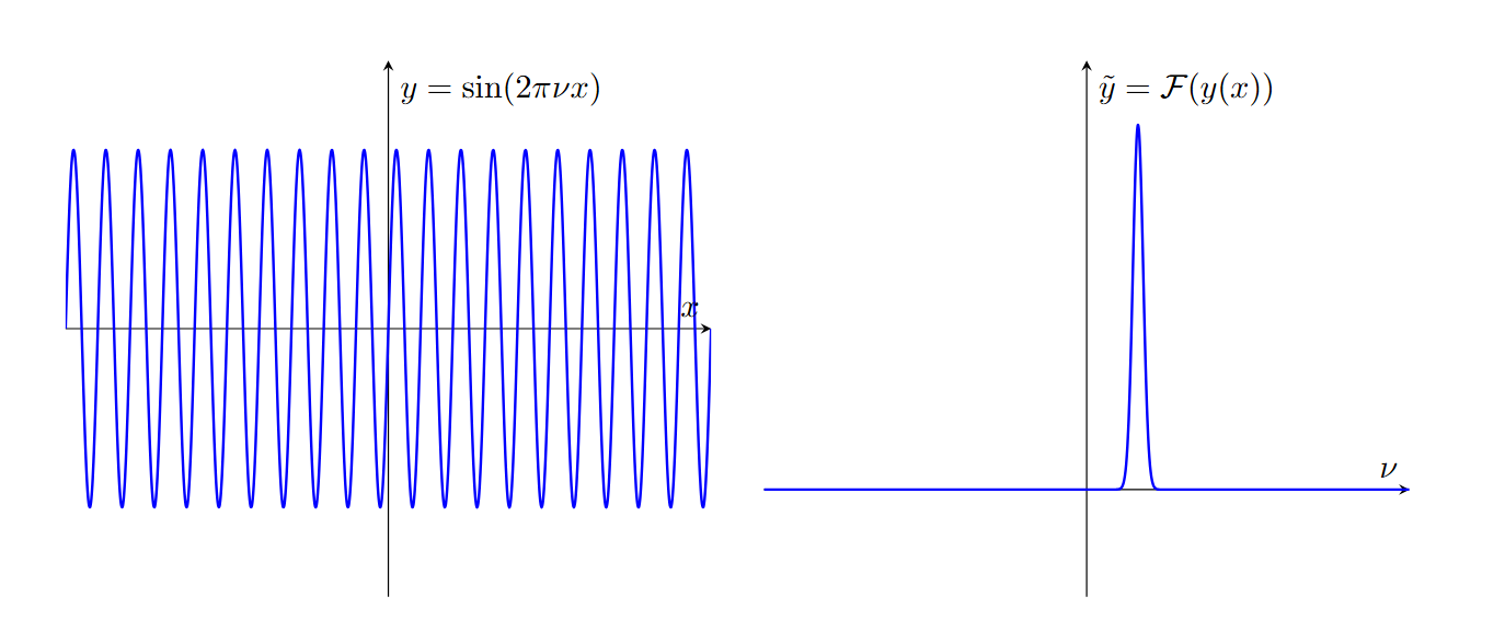
Here is an illustration for $y=\sin(2\pi\nu x)$, whose Fourier transform DFT $\tilde{y}$ has the peak at $\nu$. Note that the broadening of the unique peak occurs due to the finiteness of the data size. There is a single peak since $\sin(2\pi\nu x)$ has the fundamental mode and no additional harmonics.

Now consider the function $f(x)=a^x\mod N$ where $a\in\mathbb{Z}$ and $N\in\mathbb{N}$, which is periodic over the scales of $N$. Decomposing as a DFT, we have the following interpretation.

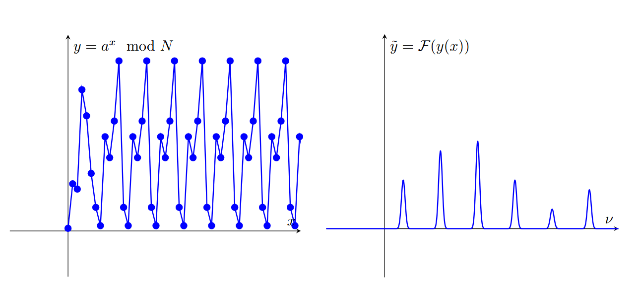
We note that the peaks of the DFT correspond to the Fourier fundamental frequencies, which are integral multiples of the period.

We generalize this idea of hunting for fundamental frequencies to a general vector by describing the DFT as the tool that decomposes a vector of complex numbers into its intrinsic frequency components. The formal definition of the algorithm is as follows:

Input: A vector of complex numbers $x_0, x_1, \dots, x_{N-1}$, where $N$ is a fixed parameter (assuming $N = 2^n$).

Output: A vector of complex numbers $y_0, y_1, \dots, y_{N-1}$, such that

\[y_k = \frac{1}{\sqrt{N}} \sum_{j=0}^{N-1} e^{2\pi i j k/N} x_j\]

Let’s build up the picture step by step. The DFT decomposes the input vector into a linear combination of complex exponentials. These exponentials, given by the factors $e^{2\pi i j k/N}$, serve as basis functions that oscillate at specific frequencies. For each $k$, we can think of $e^{2\pi i k}/N$ as a complex vector with $N$ entries, individually by \(v_k=\left(\frac 1N,\frac1N e^{2 \pi i k / N},\frac1N e^{4 \pi i k / N},\dots,\frac1N e^{2 \pi i k (N-1) / N}\right)\) These $N$ vectors form an orthonormal basis of $\mathbb{C}^N$, and can be used to decompose any vector into components along these vectors. We can directly compute the dot product of our vector to note the component along the suitable basis vector. When the input signal has a periodic structure, these basis vectors align with the natural periodicities of the signal, producing prominent peaks in the output. The term $e^{2\pi i j k/N}$ can be viewed as a rotating phase factor. For a fixed $k$, as $j$ runs over the values $0$ to $N-1$, these exponentials trace out a complete cycle. When the input signal $x_j$ resonates with this cycle (that is, when the signal contains a frequency component matching $k/N$), the sum in the above equation reinforces this frequency component, leading to a peak in the output $y_k$.

Remark: Using the Fast Fourier Transform algorithm, we can do DFT faster. We will see that during the exercise of making a Quantum Fourier Transform algorithm, FFT will appear as a byproduct.

Acknowledgement

The primary content of this post was written by Nishkal Rao. A heartfelt thank you to him for his contributions and insightful discussions!